Sabbah-Mochizuki-Kedlaya’s Hukuhara-Levelt-Turrittin Theorem

When I first started learning about irregular perverse sheaves, I struggled to find a clear answer to the question: “what does an irregular perverse sheaf look like, in the simplest cases? What should be my intuition?” If I don’t know about the motivation from differential equations, how can I picture them? This is not yet feasible given the current state of the literature; moreover, there is no general introduction to this motivation if you care about getting your hands on these new objects. Aside from the dumb name, perverse sheaves are some of the most natural objects in complex geometry, so I was hoping for a similar situation in the irregular world. This introduction doesn’t exist yet, but I hope to eventually write one.

Specifically, I was looking for analogues for the following fundamental properties:

Generically, a perverse sheaf is just a locally constant sheaf of finite rank.
The support of a perverse sheaf $\mathbf{P}^\bullet$ is a complex analytic space, and admits a Whitney stratification—a locally finite partition into complex analytic submanifolds $S$ of the ambient manifold $M$ along which the cohomology sheaves $H^k(\mathbf{P}^\bullet)_{|_S}$ are local systems, and
the normal data $\mu_\xi(\mathbf{P}^\bullet)$ is a finite dimensional vector space concentrated in a single degree, independent of $\xi \in T_S^*M$ chosen generically (this last property is sometimes called the microlocal characterization of perversity, and can be found as definition 10.3.7 in Kashiwara-Schapira’s Sheaves on Manifolds).

There are many obstacles to reaching an understanding of the appropriate analogues for irregular perverse sheaves, and I do hope to eventually cover all of them. In this post, I hope to address parts of all these things. I’ll be broadly following Sabbah’s “Recent Advances in Holonomic D-modules” and adding in some extra explanation where I needed it.

If you can get your foot in the door and get around the use of ind-sheaves and their enhancement and the instrumental role of the convolution functor $\overset{+}{\otimes}$ , then an irregular $\mathbb{R}$ -constructible (ind-)sheaf is one which, locally in the subanalytic topology on $M$ , “comes from” an ordinary $\mathbb{R}-$ constructible sheaf with a “trivial filtration” (see section 6.6 of Kashiwara-Schapira’s “Regular and Irregular Holonomic D-modules”). If you look through section 5 of Kuwagaki’s “Irregular Perverse Sheaves”, then irregular constructibility is a property that is defined after finitely many complex blow-ups to a normal crossing divisor, on the real blow-up of that divisor, in terms of irregular constant sheaves that look nothing like what your average joe topologist thinks a constant sheaf should be.

The core of the issue, alluded to in the last post, is the distinction between formal solutions and convergent solutions, and asymptotic expansions of exact solutions in terms of exponential factors (like we talked about in our brief discussion on the Airy equation). These expansions are often the most important property of the solutions, as the arise all over the place in physics (basically every time you use special functions or Fourier analysis), even if they are not the exact analytic solution. The key to understanding all of this, I believe, is Sabbah-Mochizuki-Kedlaya’s Hukuhara-Levelt-Turritin theorem.

Yes, people really call it that.

A Meromorphic connection $(M,\nabla)$ on a complex disk with a single regular singular point at $0$ has a basis of solutions given by a multivalued functions times entire functions (like $z^\alpha$ times a convergent power series, with maybe some logarithmic terms thrown in if two of the exponents $\alpha$ are repeated or differ by an integer). Under Riemann-Hilbert, these turn into perverse sheaves $DR(M,\nabla)$ where the local system in degree -1 corresponds to the flat sections $\ker \nabla$ away from 0, and the data of $DR(M,\nabla)$ is completely determined by the monodromy of these flat sections and any confluence in the eigenvalues of the exponents of the terms $z^\alpha$ . The moral of this being, the topological properties of $DR(M,\nabla)$ comes from understanding the associated ODEs, and every perverse sheaf is of this form for some $(M,\nabla)$ . Analogously, we’ll need to first understand what a basis of solutions “looks like” for irregular singularities before we can talk about their topological properties.

Our main coefficient rings in the previous two posts were the local ring $\mathscr{O}_{X,0} \cong \mathbb{C}\{z\}$ and its fraction field $\mathscr{O}_X(*0) \cong \mathbb{C}\{z\}[z^{-1}]$ . We’ll now need to introduce the formal completion of $\mathscr{O}_{X,0}$ ,

$\widehat{\mathscr{O}}_{X,0} := \varprojlim_{i \geq 1} \mathscr{O}_{X,0}/{\mathfrak{m}_{X,0}}^i \cong \mathbb{C}[[z]]$

the ring of formal power series in $z$ at 0. By considering a Meromorphic connection as a $\mathbb{C}\{z\}[z^{-1}]$ -module, we get a natural inclusion functor into the category of $\mathbb{C}[[z]][z^{-1}]$ -modules by extension of scalars. For connections with regular singularities, this map is always an isomorphism (moreover, it is an isomorphism if and only if the connection has regular singularities), proved by Malgrange in dimension 1, and Kashiwara-Kawai in general. Hence, in the irregular setting, we expect different behavior depending on whether we work over $\mathbb{C}\{z\}$ or over $\mathbb{C}[[z]]$ . The first of these differences, the place we’ll start, is the following:

Theorem(Levelt-Turrittin)

Let $(M,\nabla) \in Conn(X;\{0\})$ , and let $(\widehat{M},\widehat{\nabla})$ be its formal completion as a $\mathbb{C}[[z]][z^{-1}]$ -module. Then, there is a finite subset $latex \Phi \subseteq \mathscr{O}_{X,0}(*0)/\mathscr{O}_{X,0} \cong z^{-1}\mathbb{C}[z^{-1}]$ and an isomorphism of $\mathbb{C}[[z]][z^{-1}]$ -modules

$(\widehat{M},\widehat{\nabla}) \xrightarrow{\widehat{\lambda}} \bigoplus_{\varphi \in \Phi} \left (\mathscr{O}_X(*0)^{d_\varphi},d+d\varphi+C_\varphi \frac{dz}{z} \right)$

where $C_\varphi \in M_{d_\varphi}(\mathbb{C})$ . That is, up to formal isomorphism, a Meromorphic connection is a finite direct sum of connections with exponential factor times a connection with regular singularity. For $\varphi \in z^{-1}\mathbb{C}[z^{-1}]$ , set

$\mathcal{E}^\varphi := (\mathscr{O}_X(*0),d+d\varphi)$ .

Then, the Levelt-Turrittin theorem says that $(M,\nabla)$ is formally isomorphic to a direct sum of connections of the form $\mathcal{E}^\varphi \otimes \mathcal{R}_\varphi$ (where $\mathcal{R}_\varphi$ is a connection with regular singularity).

We’re lying a bit here, though; the full statement of the theorem is that this formal decomposition is only true after possible finite ramification of the variable $z$ . That is, if $\rho: X \to X$ sends $z \mapsto z^p$ for a positive integer $p$ , then the decomposition holds for $\widehat{\rho^*M}$ .

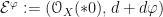
So, in the case of the Airy equation $(\partial_z^2 -z)u = 0$ with irregular singularity at infinity, the associated Meromorphic connection is formally isomorphic to

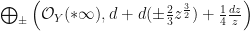
$\bigoplus_{\pm} \left (\mathcal{O}_Y(*\infty),d+d(\pm \frac{2}{3}z^\frac{3}{2})+\frac{1}{4} \frac{dz}{z} \right )$

where $Y$ is a disk around $\infty$ inside $\mathbb{P}^1$ . This sum reflects the fact that the Airy functions can be asymptotically approximated by linear combinations

$c_1 z^{-\frac{1}{4}}e^{\frac{2}{3}z^{\frac{3}{2}}}+c_2 z^{-\frac{1}{4}}e^{-\frac{2}{3}z^{\frac{3}{2}}}$ .

The issue we brought up with these approximations last post was that the exact solutions to the Airy equation are entire functions, but these exponential functions are multivalued. Hence, any such approximation cannot hold with the same values $c_1,c_2$ for all values of $z$ as it travels counterclockwise around infinity. This is generally known as the Stokes Phenomenon; the isomorphism of formal meromorphic connections guaranteed by the Levelt-Turrittin theorm does not in general lift to a global isomorphism of meromorphic connections. We can, however, locally lift the formal isomorphism on arc neighborhoods of the singular point. But, what do we mean by locally?

The Real Blow-up and Arc Neighborhoods

We want to work locally around each angle $\theta \in S^1$ , and the arc neighborhoods $S_r(a,b) = \{ z \in X | 0 < |z| < r, a < \arg z < b\}$ introduced last post are rectangular if we work in polar coordinates. The space with these coordinates is called the real oriented blowup of X at 0, denoted $\overset{\thicksim}{X} := S^1 \times [0,1)$ with natural map

$\varpi : \overset{\thicksim}{X} \to X$

$(e^{i\theta},r) \mapsto re^{i\theta}$

$\overset{\thicksim}{X}$ is not a complex manifold, so it doesn’t really make sense to talk about a sheaf of holomorphic functions on all of $\overset{\thicksim}{X}$ . But it is a real manifold with boundary, so there is a well-defined sheaf of smooth functions $\mathscr{C}_{\overset{\thicksim}{X}}^\infty$ . On the complement of boundary $\varpi^{-1}(0) \cong S^1$ , there is a natural subsheaf of holomorphic functions ${\mathscr{O}_{\overset{\thicksim}{X}}}_{|_{\overset{\thicksim}{X}-\varpi^{-1}(0)}} \cong \mathscr{O}_{X^*}$ , so the only trouble is understanding the right analogue of “holomorphic function” on the boundary. We’d like these functions to satisfy (something like) the Cauchy-Riemann equation $\partial_{\overline{z}}f(z) = 0$ and have a power series representation everywhere, even the boundary.

Is $\overline{\partial}$ even well-defined on $\overset{\thicksim}{X}$ ? Sort of. If we work in polar coordinates $(r,e^{i\theta})$ on $\overset{\thicksim}{X}$ , then a quick computation tells us that

$\overline{z}\partial_{\overline{z}} = \frac{1}{2}\left (r\partial_r+i\partial_\theta \right )$

as operators on $C_{\overset{\thicksim}{X}}^\infty$ . So, we can talk about the operator $\overline{\partial} := \partial_{\overline{z}}$ on $\widetilde X$ that acts on smooth functions and produces a smooth function with maybe a logarithmic pole at 0 (by just diving both sides of the expression by $\overline{z}$ ). So, in analogy with how on $X$ itself we can realize $\mathscr{O}_X$ as the flat sections of $C_X^\infty \xrightarrow{\overline{\partial}} C_X^\infty \otimes_{\mathscr{O}_{\overline{X}}} \Omega_{\overline{X}}^1$ , we define the sheaf of holomorphic functions on $\widetilde X$ , denoted $\mathcal{A}_{\widetilde X}$ , to be the flat sections of the connection

$C_{\widetilde X}^\infty \xrightarrow{\overline{\partial}} C_{\widetilde X}^\infty \otimes_{\varpi^{-1}\mathscr{O}_{\overline{X}}} \varpi^{-1}\Omega_{\overline{X}}^1(\log \overline{\{0\}})$ .

That is, $\ker \overline{\partial} =: \mathcal{A}_{\widetilde X}$ . If $S_\epsilon(a,b)$ (with $0 < \epsilon \ll 1$ , $a < b$ with $0 < b-a < 2\pi$ is a proper arc neighborhood of 0, then $\mathcal{A}_{\widetilde X}(S_\epsilon(a,b)) \cong \mathscr{O}_X(S_\epsilon(a,b))$ .

What does this give us? Asymptotic Expansions.

The sheaf $\mathcal{A}_{\widetilde X}$ is only really a new object for us on the boundary of $\widetilde X$ , $\varpi^{-1}(0) \cong S^1$ , so let’s focus on that. Denote ${\mathcal{A}_{{\widetilde X}}}_{|_{S^1}} = \mathcal{A}$ ; this is a subsheaf of $i^{-1}j_*\mathscr{O}_{X^*}$ . What sort of functions does it contain?

Let $e^{i\theta} \in S^1$ , and let’s look at the stalk $\mathcal{A}_{e^{i\theta}}$ , say on some small proper arc neighborhood $S_r(a,b)$ containing $\theta$ , and take a function $f \in \mathcal{A}$ defined on this neighborhood. Then, $f$ admits an asymptotic expansion at 0; that is, there is a formal series $c = \sum_{n \geq 0} c_n z^n \in \mathbb{C}[[z]]$ such that, for all $N \in \mathbb{N}$ , and every closed subsector $W \subset S_r(a,b)$ , we can find a constant $C_{N,W} > 0$ such that the estimate

$|f(z)-\sum_{n=0}^{N-1}c_n z^n| < C_{N,W}|z|^N$

holds for all $z\in W$ . We specify formal series because sometimes the functions we care about might be asymptotic to a divergent series; oftentimes power series solutions to differential equations are divergent, so we need this possibility. Poincaré developed the idea of asymptotic expansions in 1886, as a kind of analogy to Taylor series expansions of smooth functions, that still provide a useful approximation for divergent series. If $f$ is asymptotic to a series $c \in \mathbb{C}[[z]]$ above, we write $f \thicksim c$ . An example of something outside from ordinary stuff like Taylor series is

$e^{-\frac{1}{z}}\int_{1}^{1/z} \frac{e^t}{t} \, dt \thicksim \sum_{n \geq 0} n! z^{n+1}$

which clearly doesn’t converge on any neighborhood of the origin. The sheaf $\mathcal{A}$ on $S^1$ consists of all those smooth functions on $C_{\widetilde X}^\infty$ that locally admit an asymptotic expansion on the boundary of $\widetilde X$ . It contains things like $e^{-1/z}$ , but only for those $\theta \in S^1$ where $\theta \in (3\pi/2,\pi/2) \mod 2\pi$ (where $e^{-1/z} \thicksim 0$ ). It also contains all of our exponential factors $e^\phi$ whenever $\textnormal{Re}\phi < 0$ . We’ll see more later about this sheaf $\mathcal{A}_{\widetilde X}$ with moderate growth and rapid decay functions and the Borel-Ritt Lemma.

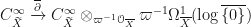
Okay, now we want to talk about differential operators up on $\widetilde X$ , and the most natural way of doing this is to set

$\mathscr{D}_{\widetilde X} = \mathcal{A}_{\widetilde X} \otimes_{\varpi^{-1}\mathscr{O}_X} \varpi^{-1}\mathscr{D}_X$

And likewise define $\mathcal{A}_{\widetilde X}(*0) = \mathcal{A}_{\widetilde X} \otimes_{\varpi^{-1}\mathscr{O}_X} \varpi^{-1}\mathscr{O}_X(*0)$ . So, tensoring with $\varpi^{-1}\mathscr{O}_X(*0)$ allows us turn meromorphic connections (which are $\mathscr{O}_X(*0)$ -modules with connection) into $\mathcal{A}_{\widetilde X}(*0)$ -modules with connection in a natural way. The point of all this is that, over $\mathcal{A}_{\widetilde X}$ , we can locally lift the formal isomorphism of the Levelt-Turrittin theorem to an isomorphism of honest-to-goodness connections.

Theorem(Hukuhara-Turrittin)

For each $e^{i\theta} \in S^1$ , the formal isomorphism $\widehat{\lambda}$ can be locally lifted as an isomorphism

$\mathcal{A}_{\widetilde X} \otimes_{\varpi^{-1}\mathscr{O}_X}(M,\nabla) \xrightarrow{\lambda_\theta} \bigoplus_{\varphi \in \Phi} \left (\mathcal{A}_{\widetilde X}(*0)^{d_\varphi},d+d\varphi+C_\varphi \frac{dz}{z} \right)$

This is exactly an algebraification of the Stokes phenomenon. The Levelt-Turrittin theorem tells us the asymptotic behavior as we approach 0 (in the form of exponential factors tensored with regular connections), and the Hukuhara-Turrittin theorem tells us that, while this behavior is true locally around $S^1 = \varpi^{-1}(0)$ , the exact description of the isomorphism may change as we travel around the circle (i.e., doesn’t necessarily give an isomorphism of $\mathscr{O}_X(*0)$ -modules). This if the reason why we can’t make a global choice of coefficients for the asymptotic expansions of exact solutions of the Airy equation.

Things are slightly more complicated in higher dimensions—these decompositions do not hold a priori hold in general without some assumptions. If we work consider meromorphic connections on a polydisk $X$ with poles along a simple normal crossings divisor $\Delta = \{z_1\cdots z_r = 0\}$ , then we have to assume that our connections have a good formal decomposition (which means that we can find a finite set $\Phi \subset \in \mathscr{O}_X(*0)/\mathscr{O}_X$ that gives such a formal decomposition, and goodness means that pairwise choices of exponential factors $\phi \neq \psi$ have divisor of zeroes $\phi - \psi$ that is empty near 0). Assuming a good formal decomposition, we can then locally lift it to a real isomorphism over $\mathcal{A}_{\widetilde X}$ (this is due to Hukuhara-Turrittin-Sibuya-Malgrange-Sabbah-Mochizuki). The goalposts are now moved to:

“when does a meromophic connection have a good formal decomposition?”

In dimension 2, Claude Sabbah conjectured that this held in general (e.g. for a general surface and divisor) after perhaps a finite sequence of point blow-ups (he proved that this was true for connections of rank $\leq 5$ ). Mochizuki was able to prove this in the projective algebraic setting in dimension 2 in 2008, and Kedlaya proved the general case in dimension 2 shortly after in 2009. Then again, Mochizuki prove the algebraic case in all dimensions, and Kedlaya proved the local analytic case in all dimensions.

Theorem (Sabbah-Mochizuki-Kedlaya, Hukuhara-Levelt-Turrittin)

Given a meromophic connection $(M,\nabla)$ on a space $X$ with poles in a divisor $D$ , and any point $x \in D$ , there is an open neighborhood $U$ of $x$ finite sequence of blow-ups $e: U^\prime \to U$ such that $e^{-1}(D) = D^\prime$ has normal crossings and $e^*(M,\nabla)$ has a good formal decomposition at each point of $D^\prime$

Right now, in a small neighborhood of this post, I’ll only be focusing on the one dimensional case, so we won’t see all these details yet. But, this data is all absolutely essential in understanding the irregular Riemann-Hilbert correspondence in this case. It tells us what to expect of the structure of “solutions” as algebraic objects, and that all of the interesting behavior happens on $\varpi^{-1}(0)$ inside the real blow-up. This is exactly the reason why irregular perverse sheaves are still generically local systems; the support condition for perverse sheaves carries through essentially unchanged to irregular perverse sheaves (modulo understanding how we embed perverse sheaves into this bigger category).

Monodromy of solutions is now a different beast; it is not determined by the multi-valuedness of the coefficients $z^\alpha$ in the solutions, it is determined by the fact that we entire exact solutions with multi-valued approximations. “Irregular monodromy” then, is the data of the family of isomorphisms $\{\lambda_\theta \}_{e^{i\theta} \in S^1}$ in the Hukuhara-Levelt theorem.

I can’t answer now all of the the broad questions I had at the beginning of this post, but this is the first step.

What comes next: the Stokes filtration. Away from the origin, the solutions of irregular holonomic D-modules are locally constant sheaves (since $\mathcal{A}_{\widetilde X}$ agrees with $j_*\mathscr{O}_{X^*}$ away from $\varpi^{-1}(0)$ ), and so the difficultly will be in understanding both the formal structure at the origin, along with the family of isomorphisms $\lambda_{\theta}$ , without knowing the exponential factors.

Sabbah-Mochizuki-Kedlaya’s Hukuhara-Levelt-Turrittin Theorem

Published by brianhepler

Leave a Reply Cancel reply

Share this:

Like this:

Related

Published by brianhepler

Leave a Reply Cancel reply